Next in super useful tools for physicists is Mathematica. If you're a physicist, I'm sure you've fiddled around a bit with Mathematica. I'll do a little intro and show how I usually utilize Mathematica.
Intro
First things first, let's do some arithmetic. You can type the same way you would a normal calculator and hit shift+enter.
![]()
![]()
Mathematica is cool and allows you to type the way you would write on paper.
We don't need the * to multiply because it can be inferred.
You can type the symbol pi by hitting esc, p, esc.
The escape key lets you type in symbols which you can find here.
You can also write exponents, square roots, and fractions using ctrl.
ctrl + 6 will type exponents ![]()
ctrl + 2 will do a square root ![]()
ctrl + /will make a fraction ![]()
Rewriting the first calculation
![]()
![]()
Much more pretty.
Variables and Functions
You can use variables to do symbolic calculations. You can also assign values to variables.
![]()
![]()
Here, I use // as an after thought to apply the function Simplify
![]()
![]()
![]()
You'll notice that assigned variables are black and unassigned variables are blue.
You can also assign variables as an after thought.
![]()
![]()
You may have noticed that I use the cosine function with square brackets. Square brackets are used for function parameters so avoid square brackets unless it is for functions.
We can define our own function with this notation.
![]()
:= is notation for delayed definition (evaluate each time the function is called).
We can now use the function.
![]()
![]()
Visualization
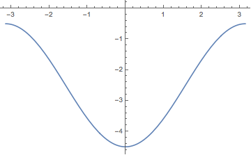
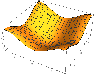
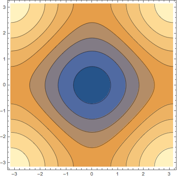
Let's try to visualize the function we just defined. There are many different ways to plot.
![]()
You can find more ways to visualize here. You can also add options to make the plot look how you want.
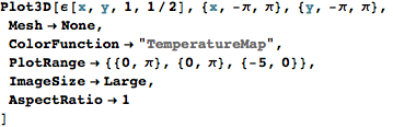
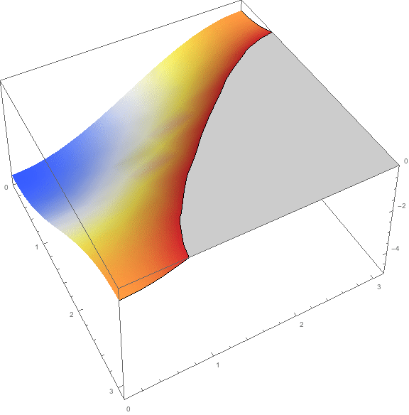
You can find these options by going to the documentation. Do this by pressing F1 with the cursor on the function.
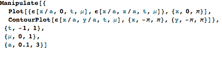
Manipulation
Here is the fun part of Mathematica. It is super easy to make interactive plots.
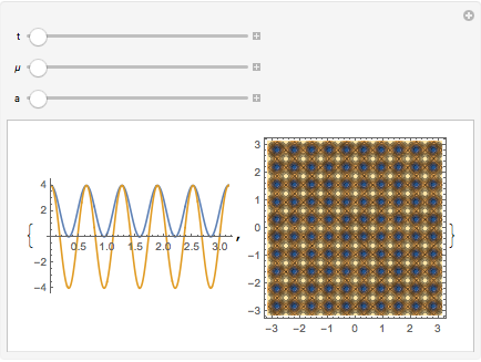
That is basically it. My main use of Mathematica is to visualize functions. If you want to learn more, you can move on but as long as you can plot functions, that's all you really need.
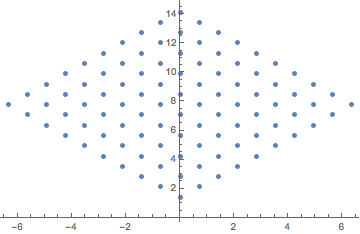
Lists
Another common need is lists which will also be used for arrays, vectors, matrices, network graphs, etc.
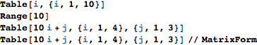
![]()
![]()
![]()

Access elements in a table with double square brackets
![]()
![]()
![]()
If you have multiple cores, you can construct tables in parallel
![]()
![]()
![]()
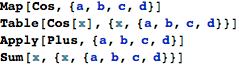
Map and Apply
List operations are made easier with map and apply. Map does element wise operation whereas apply does a collective operation.
![]()
![]()
![]()
![]()
Map and apply are so ubiquitous, it has its own notation.
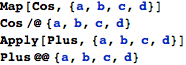
![]()
![]()
![]()
![]()
Vectors and Matrices
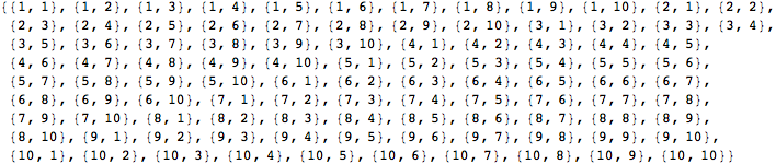
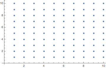
A 2D vector is just a 2 element list. Here, I make a list of coordinates.
![]()
![]()
I can now do a matrix operation on each coordinate
![]()

To review, I defined a function that takes a point. The function rotates the point 45 degrees around the origin. I then map it onto my list of points.
Pure functions
I can do the previous operation in one line with a pure function.
![]()
This is getting a little abstract and I personally don't like all this complicated syntax but you may encounter this in other people's Mathematica notebooks. Using # and & is like an anonymous function. # means the first argument. #2 can be used for the next argument. & is where the arguments are assigned.
![]()
![]()
![]()
![]()
![]()
![]()
You can find more on this here.
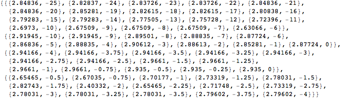
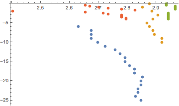
Import Data
Many times, you'll get data from a csv or xls. Mathematica is pretty good figuring out how to interpret the data.
![]()
Overlay data
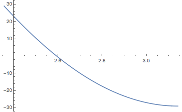
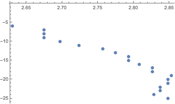
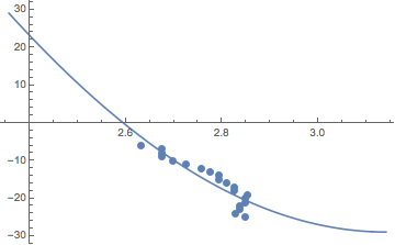
Here, I fit the ε function I defined earlier to the data. I then plot this fit and assign it the name plot1. plot2 is the list plot. By using the Show function, I can overlay these two different plots.
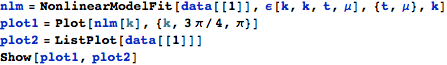
![]()
Conclusion
There are a lot of features in Mathematica. It is better to start using Mathematica and gradually learn more features. I recommend using the plot and manipulate functions first. Once you get comfortable with this, you can experiment with more features. You can learn more of the features in the online book “An Elementary Introduction to the Wolfram Language”. Here are some more functions to check out:
Integrate
Derivative
FindPeaks
Polygon
VectorPlot
GraphPlot
Histogram
N
Evaluate
Select
If you want to see some really good examples, check out the demonstrations.